Precise timing of machine code with Linux perf.
03 Apr 2019
Contents:
Subscribe to my newsletter, support me on Patreon or by PayPal donation.
I feel like writing these days, so powered by this feeling I decided to share another quite useful technique that I sometimes use. Today I will show how you can utilize Intel LBR (Last Branch Record) feature to do cycle-based timing of the code blocks. Knowing precisely how much cycles it took to execute certain number of assembly instructions, how great that would be? Want to know how? Keep on reading and you will learn. Just to tease you, look at this desired report:
  0000000000400618   movb  $0x0, (%rbp,%rdx,1)
  000000000040061d   add $0x1, %rdx
  0000000000400621   cmp $0xc800000, %rdx
  0000000000400628   jnz 0x400618

  # 5 cycles
How cool is that!
It’s just an arbitrary code snippet to give you a taste of what you’ll be able to see in this article. This shows precise number of cycles for a given basic block: 4 instructions in a block were executed in 5 cycles.
I find it very educational to look at those numbers and try to understand why you get them. Again, great for improving the mental model of how CPU works.
I want to thank Andi Kleen for showing me this technique.
Recap on LBR
The underlying CPU feature that allows this to happen is called LBR(Last Branch Record). I previously wrote an article about LBR, so I encourage you to visit this blog post if you want to know what it is.
LBR feature is used to track control flow of the program. This feature uses MSRs (Model Specific Registers) to store history of last executed branches. Why we are so interested in branches? Well, because this is how we are able to determine the control flow of our program. Since we are interested in branches which are always the last instructions in a basic blocks and all instructions in the basic block are guaranteed to be executed once, we can only focus on branches. Using this control flow statistics we can determine which path of our program (chain of basic blocks) is the hottest. This is sometimes called a Hyper Block. And there are other applications of LBR feature, see here.
Traditionally LBR entry1 has two important components: FROM_IP and TO_IP, which are basically source address of the branch and destination address. If we collect long enough history of source-destination pairs, we will be able to unwind the control flow of our program. Just like a call stack! Sounds nice and simple, right?
Starting from Haswell we already could get the information if the branch was predicted or not. There was a dedicated bit for it in the LBR entry. But since Skylake additional LBR_INFO2 component was added to LBR entry which received additional Cycle Count field:
Cycle Count - Elapsed core clocks since last update to the LBR stack.
With this new field we are able not only to get the branch history, but also to get precise timing in cycles between two taken branches. Awesome! But be aware that it only works starting from Skylake. Additionally you need to have not too old version of perf (mine is 4.15.18). Here is the commit which added this functionality in perf.
Getting cycles count with linux perf
First of all, to use this functionality with perf, LBR must be enabled:
$ dmesg | grep -i lbr
[    0.228149] Performance Events: PEBS fmt3+, 32-deep LBR, Skylake events, full-width counters, Intel PMU driver.
To demonstrate usefulness of this technique I took the example from one my previous articles about Top-Down Analysis methodology. The code has a loop with a random load that typically will miss in L3-cache and go to main memory:
#include <random>

extern "C" { void foo(char* a, int n); }

const int _200MB = 1024*1024*200;

int main() {
  char* a = (char*)malloc(_200MB); // 200 MB buffer
  for (int i = 0; i < _200MB; i++) {
    a[i] = 0;
  }

  const int min = 1;
  const int max = _200MB;
  std::default_random_engine generator;
  std::uniform_int_distribution<int> distribution(min,max);

  for (int i = 0; i < 10000000; i++) {
    int random_int = distribution(generator);
    foo(a, random_int);
  }

  free(a);
  return 0;
}
Function foo is implemented in assembly like this:
foo:
# start some irrelevant work
One_KB_of_NOPs
# finish some irrelevant work

# load that goes to DRAM
mov     rax, QWORD [rdi + rsi]
# introduce dependency chain
mov     rax, QWORD [rdi + rax]

xor rax, rax
ret
You can find complete code sample on my github.
Let’s collect LBR data on this application:
$ ~/perf record -b -e cycles ./a.out
[ perf record: Woken up 13 times to write data ]
[ perf record: Captured and wrote 3.024 MB perf.data (3864 samples) ]
Now let’s decode the data we collected. You need xed (Intel X86 Encoder Decoder) to see the instructions not just the raw bytes.
$ ~/perf script -F +brstackinsn | ../xed -F insn: -A -64 > dump.txt
Now in dump.txt we have all the branch history records, but we are only interested in those which end with return from foo instruction:
  ... <lots of code>
  400df0:       0f 1f 84 00 00 00 00    nop    DWORD PTR [rax+rax*1+0x0]
  400df7:       00
  400df8:       0f 1f 84 00 00 00 00    nop    DWORD PTR [rax+rax*1+0x0]
  400dff:       00
  400e00:       48 8b 04 37             mov    rax,QWORD PTR [rdi+rsi*1]
  400e04:       48 8b 04 07             mov    rax,QWORD PTR [rdi+rax*1]
  400e08:       48 31 c0                xor    rax,rax
  400e0b:       c3                      ret                               <== This is the branch of our interest
Let’s find something interesting in the dump using the address of our ret instruction:
  ... <lots of code>
  0000000000400df0    nopl  %eax, (%rax,%rax,1)
  0000000000400df8    nopl  %eax, (%rax,%rax,1)
  0000000000400e00    movq  (%rdi,%rsi,1), %rax
  0000000000400e04    movq  (%rdi,%rax,1), %rax
  0000000000400e08    xor %rax, %rax
  0000000000400e0b    retq                            # PRED 266 cycles 0.49 IPC
Cool! But this is just one snippet out of many. With every sample we also capture entire LBR stack which might have multiple branch records for the block that we are interested in:
$ grep "0000000000400e0b" dump.txt | grep "cycles" -c
20536
Notice we have 3864 samples, but 20536 LBR entries for our branch. On the average for every sample we had roughly 5 LBR entries that we are interested in.
Application: estimating prefetch window
Let’s see what we can do with this timing information. Let’s collect all the timings for this RET instruction. Here is the script that creates csv file from the dump:
$ grep "0000000000400e0b" dump.txt | grep "cycles" | sort > cycle_lines.txt
$ sed 's/.*PRED \(.*\) cycles.*/\1/' cycle_lines.txt > cycles.txt
$ uniq cycles.txt uniq.txt
$ cat uniq.txt | while read line ; do echo -n $line"," >> cycles.csv && grep $line cycles.txt -w -c >> cycles.csv ; done
Now, let’s plot it:
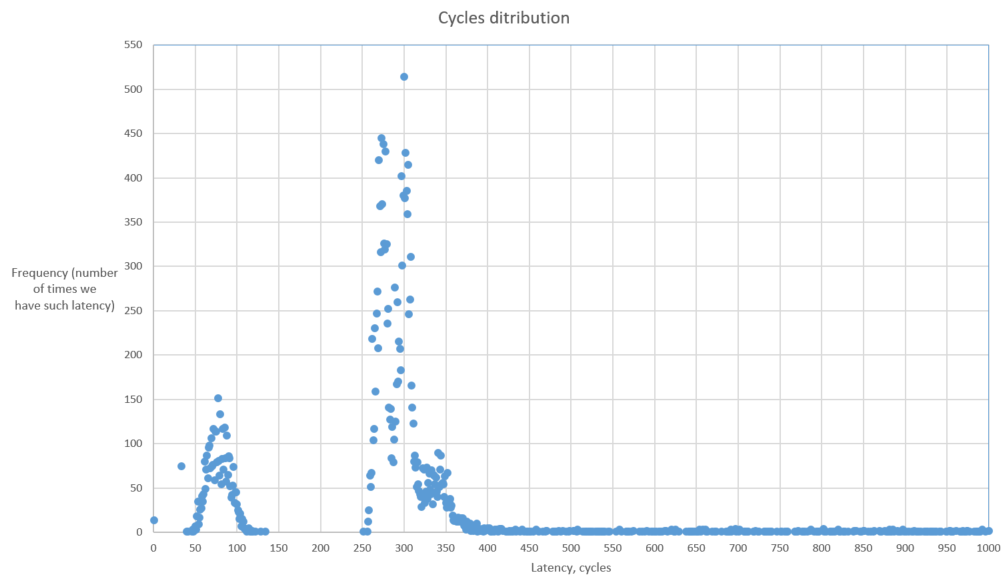
How to read this chart:
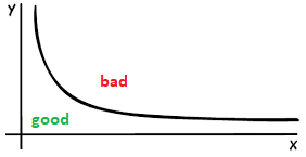
This chart shows us the number of times we got the certain latency for the basic block. On one hand we don’t want to have high latency, but on the other hand we want to have as higher amount of samples with low latency. Something like that:
To estimate prefetch window I removed both loads and collected LBR samples once again. I found that 99% of the time function foo executes in 32 cycles3. It is easy to prove since execution is bound by Retiring. On Skylake we can retire 4 instructions per cycle. In 1 KB of 8-byte NOPs we have 2^10 / 8 = 2^7 instructions. Thus it executes in 2^7 / 4 = 32 cycles.
So, this tells us that we have prefetch window of 32 cycles. In the presented case it’s constant and doesn’t vary, but in the code that you might be dealing with it likely won’t be so.
Let’s insert prefetch hint and plot the latencies for this case:
  for (int i = 0; i < 100000000; i++) {
    int random_int = distribution(generator);
+   __builtin_prefetch ( a + random_int, 0, 1);
    foo(a, random_int);
  }
Here is combined plot with original (baseline) and improved (prefetched) cases:
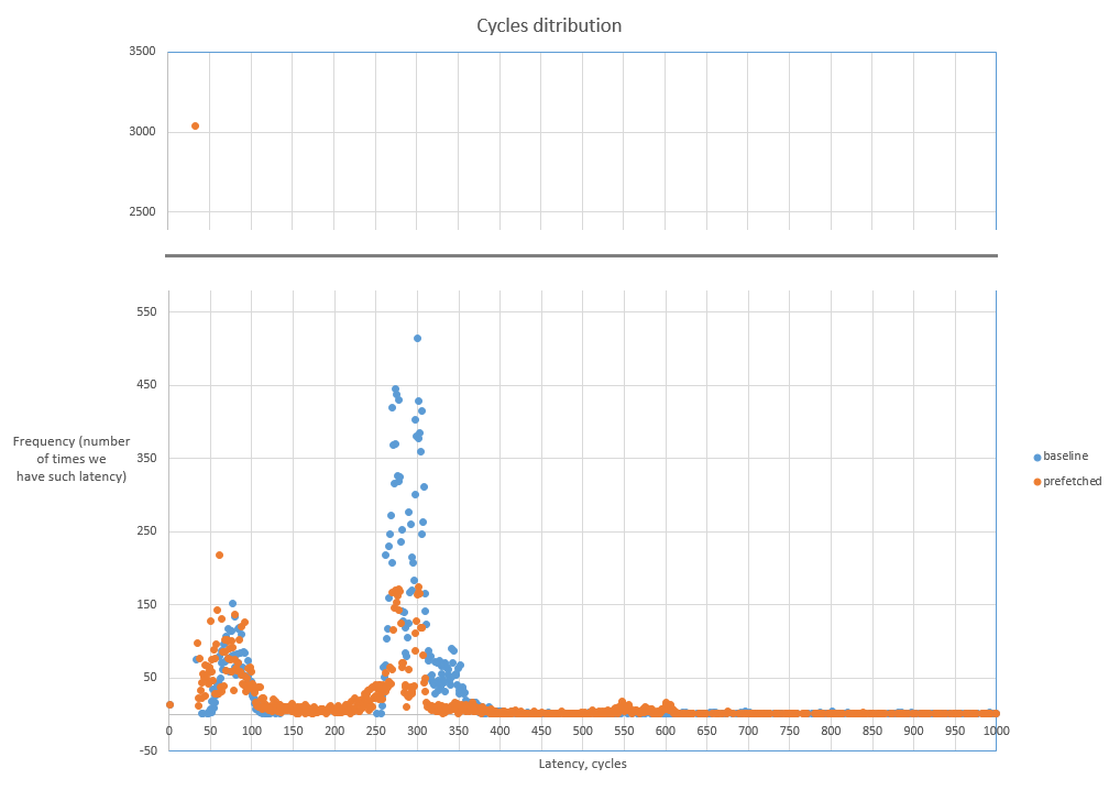
You see, we lowered the spike around 300 cycles and shifted both spikes to the left which is good (towards lower latencies). Also notice the orange dot for 32 cycles latency which has frequency around 3000 times. That means we now have much less cycles that are wasted due to demanding load that misses in caches. See more details about cache misses statistics for this exact case in my previous article about Top-Down Analysis methodology.
That’s all. Hope you enjoyed and found it useful! Good luck in using this powerful feature!
-
See https://software.intel.com/sites/default/files/managed/7c/f1/253669-sdm-vol-3b.pdf, chapter “17.4.8 LBR Stack” ↩
-
See https://software.intel.com/sites/default/files/managed/7c/f1/253669-sdm-vol-3b.pdf, chapter “17.12.1 MSR_LBR_INFO_x MSR” ↩
-
Function
foois a single basic block function, so it doesn’t matter. Same timing applies to the basic block and the whole function itself. ↩
All content on Easyperf blog is licensed under a Creative Commons Attribution 4.0 International License